04 - Transport Layer
Problem 1: Short Answer Questions
- (a) Is it possible for an application to enjoy reliable data transfer even when the application runs over UDP? If so, how?
Solution
Yes — but not from UDP itself. UDP is connectionless and provides no reliability, ordering, or retransmissions. Applications can build reliability at the application layer (e.g., add sequence numbers, acknowledgements, retransmission timers, and reassembly) on top of UDP to achieve reliable delivery semantics when needed.
Elaboration: This exemplifies the layered architecture of networking. While UDP provides a simple, lightweight service, complex reliability mechanisms (like those in TCP) can be implemented as application logic. Examples include: custom protocols for online games using UDP with selective retransmission, real-time streaming apps that detect and recover from losses, or file-transfer applications that add their own acknowledgment-based flow control.
- (b) Consider an application that issues send(sock, buffer, 5000, destinationAddress) over the UDP socket “sock”. Assuming the MTU of the Link Layer is 1500 bytes, IP header is 20 bytes, and the UDP header is 8 bytes, (1) how many IP packets are transmitted. (2) What’s the size of each packet? (3) Assuming that the 1st IP packet is lost during transmission, how many bytes does the receiver application receive if it issues recv(sock, buffer, 5000)?
Solution
- MTU payload per IP fragment for the UDP datagram: 1500 − 20 − 8 = 1472 bytes.
- 5000 / 1472 ≈ 3.39 → 4 IP packets total: 3 full fragments and 1 remainder.
- Packet sizes:
- 3 packets carry 1472 bytes of UDP payload each → 1472 + 20 (IP) + 8 (UDP) = 1500 bytes total.
- 1 packet carries 584 bytes of UDP payload → 584 + 20 + 8 = 612 bytes total.
- If the first IP fragment is lost, IP cannot reassemble the UDP datagram; the entire datagram is discarded, so the receiver’s
recv(..., 5000)returns 0 bytes for that send.
Elaboration: This illustrates the atomicity of UDP datagrams: IP fragmentation reassembly is all-or-nothing at the IP layer. If any fragment is lost, the entire datagram is dropped and the application receives nothing—there is no partial delivery. This contrasts with TCP, which operates as a byte stream where lost segments are retransmitted independently. This is why UDP works well only in contexts where occasional complete losses are acceptable (e.g., streaming media).
- (c) Consider a UDP application that runs over a virtual-circuit switched network such as ATM. This application first sends packet 1 and then packet 2 to the receiver. The receiver claims that it received packet 2 before packet 1. Is the receiver telling the truth, or is it lying? Why or why not.
Solution
Lying (under normal assumptions). Although UDP itself is unordered, a virtual-circuit network preserves per-circuit ordering. If both packets were sent on the same VC, the network guarantees in-order delivery, so packet 1 should arrive before packet 2.
Elaboration: Virtual-circuit networks (like ATM) establish a fixed path through the network and maintain per-VC state at each router. This ensures that all packets on that VC traverse the same sequence of routers and links, preserving FIFO order. In contrast, datagram networks (like IP) can route each packet independently, potentially allowing out-of-order arrival. The ordering guarantee is a property of the network layer, not the transport layer (UDP).
- (d) Consider a UDP application that wants to broadcast a UDP packet to all nodes attached to the same link. What would be the destination IP and destination MAC address of the packet sent?
Solution
- Destination MAC: FF:FF:FF:FF:FF:FF
- Destination IP: 255.255.255.255 (limited broadcast) or the subnet-directed broadcast for the link.
Elaboration: Broadcasting requires special addresses at both the network and data-link layers. The MAC address FF:FF:FF:FF:FF:FF is the link-layer broadcast address—all devices on the link listen to it. For IP, 255.255.255.255 is a limited broadcast (not routed; stays on the local network), while X.X.X.255 (in subnet X.X.X.0/24) is a directed broadcast (routed to a specific subnet). Routers typically filter directed broadcasts for security reasons, so limited broadcast is more commonly used.
- (e) Consider a UDP server that binds itself to the UDP port 80 at an interface having IP address $IP_1$. Consider a UDP client with IP address $IP_2$ and port number 2000. What would be <SrcIP, DestIP><SrcPort, DestPort> of the packets sent from the client to the server?
Solution
<$IP_2$, $IP_1$><2000, 80>
Elaboration: UDP is connectionless, so each packet explicitly carries the full 4-tuple (source IP, source port, destination IP, destination port). The source fields reflect the client’s identity ($IP_2$, port 2000), and the destination fields target the server ($IP_1$, port 80). The server, upon receiving this packet, will identify which application to deliver it to based on the destination port and can respond by swapping source and destination fields.
- (f) Assume that you run UDP over a network that employs reliable-delivery at the network layer (e.g., X.25). Would any of the packets sent by your UDP sender be lost within the network? Why or why not?
Solution
With a reliable network layer (e.g., X.25), packets shouldn’t be lost within the network path. However, UDP still provides no end-to-end recovery or ordering; reliability is not guaranteed unless the application adds it.
Elaboration: Network-layer reliability (hop-by-hop retransmission) ensures packets traverse the core network intact but does not protect against losses at the endpoints, errors in the last-mile link, or application-level buffer overflows. Additionally, reliability at lower layers does not automatically translate to end-to-end transport semantics—only UDP’s behavior (no retransmissions, no ordering) is guaranteed. An application still needs to handle out-of-order arrivals or implement its own end-to-end checks if full reliability is required.
- (g) Describe why an application developer may choose to run an application over UDP rather than TCP?
Solution
Lower latency and smaller headers; no connection setup; multicast/broadcast support; and freedom to implement custom reliability, ordering, or timing policies in the application. Good for real-time or fault-tolerant media.
Elaboration: TCP’s 3-way handshake adds initial latency, and congestion control/flow control mechanisms can delay data transmission to ensure fairness and network stability—unacceptable for delay-sensitive applications. UDP’s 8-byte header is also smaller than TCP’s 20 bytes. More importantly, UDP allows selective retransmission policies (e.g., discard stale video frames) and multicast/broadcast, which TCP cannot support. Online games, VoIP, and video streaming exploit these properties: a few lost packets are preferable to the latency and buffering introduced by TCP’s strict reliability guarantees.
- (h) Consider a TCP connection with an MSS of 1460. Assume that the application issues a send request for 5000 bytes. How many IP packets are sent? What’s the size of each IP packet including the IP header. Assume IP header is 20 bytes and TCP header is 20 bytes.
Solution
- MSS = 1460 bytes of TCP payload.
- 5000 / 1460 ≈ 3.42 → 4 TCP segments: 3 × 1460 and 1 × 620 bytes payload.
- IP packet sizes (payload + headers):
- 3 packets: 1460 + 20 (TCP) + 20 (IP) = 1500 bytes.
- 1 packet: 620 + 20 + 20 = 660 bytes.
Elaboration: MSS (Maximum Segment Size) is negotiated during the TCP 3-way handshake and typically set to MTU − IP header − TCP header (1500 − 20 − 20 = 1460). TCP respects this limit to avoid IP fragmentation. Unlike UDP, which sends entire datagrams as single units, TCP can split application data across multiple segments—the receiver reassembles them transparently into a byte stream. This allows pipelining: the sender can transmit multiple segments before waiting for acknowledgments.
- (i) Why is it sometimes necessary to fragment a TCP packet even though it is shorter than the maximum allowed length of (65,495 bytes)?
Solution
Because the limiting factor is the link MTU along the path (e.g., Ethernet 1500 bytes). Even if the TCP segment is below 65,535 bytes, it may exceed a path MTU and must be fragmented (by IP) or segmented appropriately to traverse the link.
Elaboration: The TCP segment size is constrained by the path MTU (the smallest MTU of all links along the route), not the maximum IP datagram size. TCP uses MSS to stay within the path MTU; the IP layer will fragment any datagram exceeding a link’s MTU. Fragmentation adds overhead and complexity: fragments must be reassembled at the destination, and loss of any fragment causes the entire IP datagram to be discarded. This is why path MTU discovery is important—TCP can discover the minimum MTU and set MSS accordingly, minimizing fragmentation.
- (j) Ethernet computes a CRC to check for bits errors that may occur to the packet during transmission. Given that this is the case, why do UDP and TCP have a checksum to protect the payload?
Solution
End-to-end protection across all networks: not every link layer uses CRC, errors can occur beyond the link (e.g., in routers), and IPv6 has no header checksum. Transport checksums (over header + data + pseudo-header) provide end-to-end integrity.
Elaboration: Link-layer CRCs (e.g., Ethernet FCS) protect data only during transmission on that particular link; they are recomputed and replaced at each hop. Errors in router memory, software bugs, or bit flips in intermediate systems can corrupt packets undetected by the link CRC. Furthermore, some networks lack CRCs entirely. Transport-layer checksums, by contrast, span the entire path from source to destination and cover the transport header (which may be modified in transit) and application data. The pseudo-header (source IP, destination IP, protocol number) is also included to catch misdelivery errors where a packet is routed to the wrong host.
- (k) TCP supports having a receiver set its receive window size to zero, why might a receiver do this?
Solution
To apply flow control: advertise a zero window when its receive buffer is full to stop the sender. The sender will perform zero-window probing until the window opens again.
Elaboration: The receive window is the mechanism by which a receiver tells the sender how much unacknowledged data it can accept. When the application is slow or temporarily busy and the receive buffer fills up, the receiver advertises a window of 0, halting further transmissions. The sender respects this by not sending new data (only sending zero-window probes to check when the window reopens). This prevents buffer overflow at the receiver and provides backpressure, allowing the receiver to pace the sender without requiring the sender to detect timeout or loss.
- (l) TCP supports sending packets with zero length, why might this be useful?
Solution
For pure ACKs and control segments (e.g., SYN/FIN, keep-alives) without application payload, allowing state management and acknowledgements independent of data transfer.
Elaboration: Not every TCP segment carries application data. Pure acknowledgment segments (ACKs) confirm receipt of prior data without sending new bytes. Control segments (SYN, SYN-ACK, FIN) establish or close connections. Keep-alive probes detect broken connections by sending zero-byte segments after idle periods. Delayed ACKs and window updates may also be sent as zero-length packets. These segments are essential for protocol operation but would be wasteful if forced to carry a minimum payload. Zero-length support keeps the protocol flexible and efficient.
- (m) Why does a TCP connection start from a random starting sequence number? Briefly describe.
Solution
To mitigate off-path guessing attacks and to distinguish new data from old delayed duplicates. Random ISNs reduce spoofing risks and help avoid accepting stale segments.
Elaboration: An attacker who knows or guesses the sequence number space could inject packets into an existing TCP connection (known as a TCP injection attack). By randomizing the initial sequence number (ISN) for each new connection, an attacker must blindly guess from a 32-bit space, making injection effectively impossible. Additionally, segments from a previous connection (due to network delays or software bugs) could be mistaken for data from a new connection if sequence numbers were reused immediately; randomization helps prevent this confusion and ensures that stale segments are properly identified and discarded.
- (n) Consider a network that uses virtual circuits. Assume that you run TCP over this network and establish a connection to a server. Further assume that during the lifetime of this TCP connection, one of the routers in the network on the path to the destination crashes, and reboots back up. Would your TCP endpoints be able to continue exchanging packets, or is it necessary to close this TCP connection and establish a new connection to continue communicating? Why or why not?
Solution
In a VC network, routers keep per-connection state. If a router crashes and VC state is lost, the path is broken; the VC typically must be re-established before TCP can continue, often requiring new connection setup.
Elaboration: Virtual-circuit networks pre-establish a dedicated path through the network, with each router maintaining state (a VC ID or label) to forward packets along that path. When a router crashes, this per-connection state is lost. Upon reboot, the router has no record of which VC was being used or where to forward its traffic. TCP above sees this as a broken connection—packets cannot flow. The VC must be signaled again (via ATM or other VC setup protocols), which effectively requires re-establishing the TCP connection. In contrast, datagram networks like IP maintain no per-connection state in routers, so they can reroute packets around the crashed router transparently.
- (o) Consider a network that uses datagram switching. Assume that you run TCP over this network and establish a connection to a server. Further assume that during the lifetime of this TCP connection, one of the routers in the network on the path to the destination crashes, and reboots back up. Would your TCP endpoints be able to continue exchanging packets, or is it necessary to close this TCP connection and establish a new connection to continue communicating? Why or why not?
Solution
With datagram switching, routing can reconverge around failures without per-flow state. TCP endpoints can often continue using the same connection once paths recover, with no need to re-establish at the transport layer.
Elaboration: Datagram networks (like the Internet) have routers make independent, per-packet routing decisions based on destination IP and routing tables—no per-flow state is maintained. When a router crashes and reboots, its routing tables are rebuilt (via dynamic routing protocols like OSPF or BGP), and traffic is rerouted around the failure. From TCP’s perspective, some packets may be delayed or lost (triggering retransmission), but the connection itself remains valid. Once routing reconverges and paths are restored, TCP can resume sending and receiving normally. This resilience without connection-level re-establishment is a key advantage of datagram networks over VC networks.
- (p) True/False: TCP checksum is computed only over the TCP header.
Solution
False. TCP checksum covers the TCP header and data plus the IP pseudo-header.
Elaboration: The TCP checksum is computed over three components: (1) the TCP header, (2) the application data, and (3) a pseudo-header derived from the IP header (source IP, destination IP, protocol number, and segment length). This comprehensive coverage ensures detection of errors throughout the entire segment and also protects against misrouting—if a segment is sent to the wrong IP address, the checksum (which includes both $IP_s$) will fail. The pseudo-header is not transmitted; it is reconstructed at the receiver for checksum verification, binding the TCP segment to its intended endpoints.
- (q) True/False: RcvWindow field in the TCP segment is used for Flow Control.
Solution
True. The advertised receive window controls how much the sender may have unacknowledged in flight, preventing receiver buffer overflow.
- (r) Suppose that the last SampleRTT in a TCP connection is equal to 1 sec. Then the current value of TimeoutInterval for the connection will necessarily be greater than 1 sec. Justify your answer. A simple yes/no is NOT acceptable.
Solution
Not necessarily. TCP sets
TimeoutInterval = EstimatedRTT + 4·DevRTT. Even if the most recentSampleRTTis 1 s, theEstimatedRTTmay be below or above 1 s depending on history, andDevRTTmay be small. The interval must be ≥ the true RTT to avoid premature timeouts, but it is not guaranteed to be strictly > 1 s.Elaboration: TCP’s adaptive timeout mechanism uses exponential smoothing to estimate RTT and variance. EstimatedRTT is a weighted average of past samples, so one high sample doesn’t immediately dominate. DevRTT measures variance—on stable paths, DevRTT is small, so the timeout stays close to EstimatedRTT. The 4×DevRTT safety margin ensures timeouts occur only when packets are truly lost, not just delayed. This adaptive approach prevents spurious retransmissions on variable-delay paths while maintaining responsiveness.
- (s) Suppose host A sends over a TCP connection to host B one segment with sequence number 38 and 4 bytes of data. In the same segment the ACK number is necessarily 42. A simple YES/NO is NOT acceptable. Justify your answer.
Solution
Not necessarily. In a segment sent by A, the ACK field acknowledges data A has received from B (piggyback ACK) and is independent of A’s own
seq=38and 4‑byte payload. If B sends an ACK in response to receiving bytes 38–41 from A, that ACK number would be 42; but the ACK number carried by A in the same segment reflects the next byte A expects from B, which may be unrelated to 42.Elaboration: This illustrates TCP’s bidirectional, full-duplex nature. Each segment can simultaneously carry new data (sequence number) and acknowledge received data (ACK number) from the opposite direction. The sequence and ACK numbers operate in independent spaces—A’s outgoing sequence reflects A’s data stream to B, while A’s outgoing ACK reflects B’s data stream to A. This piggyback acknowledgment reduces protocol overhead by combining data and control information in a single packet, improving efficiency on interactive connections.
- (t) Consider a TCP sender with a slow start threshold (ssthresh) value of 14 and congestion window (cwnd) size of 20. Assuming that the sender detects a packet loss by a timeout, what are the new values of ssthresh and cwnd?
Solution
Timeout implies multiple losses. Set
ssthresh = cwnd/2 = 10andcwnd = 1 MSS(slow start).Elaboration: A timeout is considered a severe congestion signal, worse than fast retransmit (3 duplicate ACKs). Timeouts typically indicate multiple packet losses or significant network problems, suggesting the network is heavily congested. TCP responds aggressively by halving the slow-start threshold (ssthresh = cwnd/2) and resetting the congestion window to 1 MSS, forcing a return to slow-start phase. This conservative approach allows TCP to probe network capacity cautiously after suspected congestion collapse, ensuring network stability.
- (u) True/False: Host A is sending host B a large file over a TCP connection. Assume host B has no data to send to host A. Host B will not send any ACKs to host A. Justify your answer.
Solution
False. TCP always sends ACKs to confirm received data, even when the receiver has no application data to send.
Elaboration: TCP’s reliability mechanism requires explicit acknowledgment of all received data, regardless of whether the receiver has data to send back. Pure ACK segments (zero-length payloads) are essential for flow control, congestion control, and ensuring the sender knows data arrived safely. Even in asymmetric communication (like web browsing, where clients send small requests and servers send large responses), the client must ACK the server’s data to maintain TCP’s sliding window and enable proper retransmission if needed.
- (v) True/False: The size of the TCP RcvWindow never changes throughout the duration of the connection. Justify your answer.
Solution
False. The advertised receive window varies with buffer occupancy: it shrinks as data arrives and grows as the application consumes buffered data.
Elaboration: The receive window is a dynamic flow control mechanism that reflects real-time buffer availability at the receiver. As the receiver buffers incoming data waiting for the application to read it, the available space decreases, and the advertised window shrinks accordingly. When the application reads data from the buffer, space becomes available again, and the window size increases in subsequent ACKs. This provides automatic backpressure: a slow application naturally reduces the sender’s transmission rate without requiring explicit application-level coordination.
- (w) True/False: Suppose host A is sending host B a large file over a TCP connection. The number of unacknowledged bytes that A sends cannot exceed the size of the receive buffer. Justify your answer.
Solution
True. The sender is limited by the receiver’s advertised window (flow control), which reflects available buffer space.
Elaboration: TCP’s flow control prevents sender-induced buffer overflow at the receiver. The advertised window field in each ACK tells the sender exactly how much additional data the receiver can accept. The sender maintains a count of unacknowledged bytes and ensures this never exceeds the last advertised window size. This creates a sliding window where the sender can transmit up to the window limit, then must wait for ACKs (which free up space) before sending more data. This mechanism automatically adapts to receiver processing speed and available memory.
- (x) True/False: Suppose host A is sending a large file to host B over a TCP connection. If the sequence number for a segment of this connection is m, then the sequence number for the subsequent segment will necessarily be m+1.
Solution
False. TCP is a byte stream: the next segment’s sequence number is
m + (payload length). It equalsm + 1only when the current segment carries 1 byte.Elaboration: TCP’s byte-stream abstraction means sequence numbers refer to byte positions in the stream, not packet numbers. Each byte has a unique sequence number, so a segment carrying 1460 bytes advances the sequence number by 1460. This differs from packet-based protocols where sequence numbers increment by 1 per packet. The byte-stream model allows TCP to flexibly segment and reassemble data: the application can send any amount of data, and TCP can break it into optimally-sized segments for the network path without the application needing to know packet boundaries.
- (y) True/False: With the selective-repeat protocol, it is possible for the sender to receive an ACK for a packet that falls outside of its current window. Justify your answer.
Solution
True. SR acknowledges individual packets; delayed or out-of-order ACKs for packets already outside the current window can still arrive. The sender will ignore ACKs that don’t correspond to outstanding packets.
Elaboration: In Selective Repeat, each packet is individually acknowledged, and ACKs can arrive out of order due to network delays or multiple paths. Consider a sender with window [1,2,3,4]; if packets 1-3 are ACKed and the window advances to [4,5,6,7], a delayed ACK for packet 1 might still arrive. The sender recognizes this ACK as outside the current window (for an already-acknowledged packet) and ignores it safely. This robustness to delayed ACKs is crucial for protocol correctness on networks with variable delay or packet reordering.
- (z) True/False: With Go-Back-N, it is possible for the sender to receive an ACK for a packet that falls outside of its current window. Justify your answer.
Solution
True. GBN uses cumulative ACKs; duplicate or delayed ACKs for already-acknowledged (older) sequence numbers may arrive after the window has advanced and thus fall outside the current window.
Elaboration: Go-Back-N’s cumulative acknowledgment means ACK(n) confirms receipt of all packets up to n. If the sender’s window advances based on ACK(5), a later-arriving duplicate ACK(3) or ACK(4) falls outside the current window. This can happen when multiple ACKs are in flight or when the receiver sends duplicate ACKs for out-of-order packets. The sender simply ignores these outdated ACKs since they provide no new information. GBN’s simplicity in handling such cases (compared to SR’s per-packet tracking) is one reason it’s easier to implement correctly.
Problem 2: UDP Service Model
What’s the service model exported by UDP to the application programs. When would you use this service model?
Solution
UDP provides a connectionless, unreliable, unordered datagram service with no flow or congestion control. Use it for latency-sensitive or application-tolerant workloads (e.g., streaming, VoIP, DNS) where the app can handle loss/reordering or add its own lightweight reliability.
Elaboration: UDP’s simplicity makes it ideal for applications where speed matters more than perfect delivery. Each datagram is independent and self-contained, so the sender needn’t establish a connection or maintain per-flow state at the receiver. The trade-off is that applications must implement their own reliability mechanisms if needed. Streaming applications often accept occasional packet loss (resulting in audio/video glitches) because the alternative—TCP’s retransmission delays—would cause unacceptable buffering and latency. DNS queries use UDP because most names resolve on the first try; if a response is lost, the client simply retransmits the query.
Problem 3: TCP Service Model
What’s the service model exported by TCP to the application programs. When would you use this service model?
Solution
TCP provides a reliable, ordered, byte-stream, connection-oriented service with flow and congestion control. Use it when correctness and in-order delivery matter (e.g., HTTP, file transfer, email, DB protocols).
Elaboration: TCP’s comprehensive reliability guarantees come at the cost of complexity and latency. The 3-way handshake establishes a connection before data transfer; retransmission and flow control add overhead. However, for applications where data integrity is critical—file downloads, database queries, email—these costs are acceptable. The byte-stream abstraction hides packet boundaries from the application, allowing the sender to transmit any amount of data and the receiver to reassemble it in order transparently. Congestion control ensures that TCP flows share network resources fairly, preventing any single connection from monopolizing bandwidth.
Problem 4: Video Streaming Protocol Selection
Consider an application where a camera at a highway is capturing video of the passing cars at 30 frames/second and sending the video stream to a remote video viewing station over the Internet. You are hired to design an application-layer protocol to solve this problem. Which transport-layer protocol, UDP or TCP, would you use for this application and why? Justify your answer.
Solution
UDP. Real-time video tolerates some loss and out-of-order frames; avoiding retransmissions and head-of-line blocking reduces latency. The application can add minimal FEC or selective repair as needed.
Elaboration: Live video streaming presents a unique trade-off: losing a frame or two is preferable to displaying outdated video due to retransmission delays. TCP’s reliability guarantees introduce two problems: (1) timeouts and retransmissions cause playback buffering and latency spikes, and (2) if a frame arrives after the viewer has moved past that frame’s timestamp, displaying it causes visually jarring “out-of-order” frames. UDP avoids these by discarding lost frames, keeping the stream live. Modern streaming protocols (like those in WebRTC) run over UDP and employ lightweight redundancy (e.g., forward error correction) to repair occasional losses without the overhead of full TCP-style reliability. Some video systems (e.g., RTMP over TCP) do use TCP, but typically for non-interactive or pre-recorded content where latency is less critical.
Problem 5: UDP Socket Address and Port Handling
Suppose a UDP server creates a socket and starts listening for UDP packets at UDP port 5000 at host interface having IP address $IP_S$.
- (a) Suppose that a client A with IP address $IP_A$ and UDP port 2000 sends a UDP packet having a destination address $IP_S$ and destination port 5000. What’s the source and destination IP addresses and source and destination port numbers of this UDP packet? Assuming that the packet is delivered to the host where the server is running, would the UDP layer at the server deliver this packet to the UDP server?
Solution
SrcIP=$IP_A$, DestIP=$IP_S$; SrcPort=2000, DestPort=5000. Yes—demultiplexing by destination port matches the server’s bound socket.
Elaboration: UDP demultiplexing is simpler than TCP: packets are delivered to the socket bound to the destination port, regardless of source. The server socket listening on port 5000 will receive this packet because the destination port (5000) matches. UDP doesn’t maintain per-connection state, so the same server socket can receive packets from multiple clients. The server application distinguishes clients by examining the source IP and port from each received packet, allowing it to respond appropriately.
- (b) Suppose now that a client B with IP address $IP_B$ and UDP port 8000 sends a UDP packet having a destination address $IP_S$ and destination port 5000. What’s the source and destination IP addresses and source and destination port numbers of this UDP packet? Assuming that the packet is delivered to the host where the server is running, would the UDP layer at the server deliver this packet to the UDP server?
Solution
SrcIP=$IP_B$, DestIP=$IP_S$; SrcPort=8000, DestPort=5000. Yes—the server listens on port 5000 regardless of client address/port.
Elaboration: This demonstrates UDP’s connectionless nature: the server socket bound to port 5000 accepts packets from any source, as long as the destination port matches. Client B (using port 8000) can communicate with the same server as Client A (using port 2000) without interference. The OS delivers both clients’ packets to the same server application, which can differentiate them by source address. This many-to-one communication model makes UDP ideal for server applications handling multiple independent clients.
- (c) If the UDP server wants to send a UDP packet to client A described in (a) what would be the source and destination IP addresses and source and destination port numbers of the packet?
Solution
SrcIP=$IP_S$, DestIP=$IP_A$; SrcPort=5000, DestPort=2000.
Elaboration: The server responds by swapping source and destination fields from the received packet. The server’s source port (5000) becomes the response’s source, and client A’s original source port (2000) becomes the destination. This address swapping is a common pattern in UDP applications: the server uses the source information from incoming packets to determine where to send responses. Since UDP is connectionless, each response is an independent datagram with explicit addressing.
- (d) If the UDP server wants to send a UDP packet to client B described in (b) what would be the source and destination IP addresses and source and destination port numbers of the packet?
Solution
SrcIP=$IP_S$, DestIP=$IP_B$; SrcPort=5000, DestPort=8000.
Elaboration: Similar address swapping applies for client B: the server sends its response using client B’s source information ($IP_B$:8000) as the destination. This shows how a single UDP server can maintain “conversations” with multiple clients by remembering source addresses from incoming packets. Although UDP itself is stateless, applications can layer session semantics on top by tracking client addresses and maintaining per-client state as needed.
Comment on UDP's connectionless demultiplexing model
This problem illustrates UDP’s connectionless demultiplexing model. Unlike TCP, which identifies a connection by the 4-tuple (source IP, source port, destination IP, destination port) and maintains per-connection state, UDP simply listens on a specific port and accepts datagrams from any source. The server can distinguish clients by examining the source address and port of each incoming datagram, but UDP itself does not enforce connection semantics—it’s the application’s responsibility to parse packet contents and handle any client-specific logic.
Problem 6: TCP Port Numbers Bidirectional
Consider a TCP connection between host A and host B.
Suppose that the TCP segments travelling from host A to host B have source port number x and destination port number y. What are the source and destination port numbers for the segments travelling from host B to host A?
Solution
SrcPort=y, DestPort=x (the ports swap direction across the connection).
Elaboration: This symmetry reflects TCP’s point-to-point connection model. Each connection is identified by an unordered pair of endpoints: (A:x, B:y). From A’s perspective, it sends to B:y using its local port x. From B’s perspective, it sends back to A:x using its local port y. This symmetry is essential for TCP to demultiplex return traffic correctly at each end. Unlike UDP, where the server typically uses a well-known port and clients use ephemeral ports, TCP requires port symmetry to maintain bidirectional communication on a single connection.
Problem 7: Telnet Multiple Clients Port Assignment
Suppose client A initiates a Telnet session with server S. At about the same time, client B initiates a Telnet session with server S. (Recall that a Telnet session runs over TCP and a Telnet server waits for client connections at TCP port 23.) Provide possible source and destination port numbers for:
- (a) The segments sent from A to S.
Solution
SrcPort=ephemeral (e.g., 3000), DestPort=23.
Elaboration: Telnet clients use ephemeral (temporary) ports assigned by the OS, typically from a high-numbered range (32768-65535 on Linux). The destination port 23 is Telnet’s well-known service port. Using ephemeral source ports allows multiple Telnet clients on the same host to connect to different servers simultaneously, since each connection gets a unique source port. The OS automatically selects an available ephemeral port when the client creates its socket.
- (b) The segments sent from B to S.
Solution
SrcPort=ephemeral (e.g., 3001), DestPort=23.
Elaboration: Client B receives a different ephemeral port (3001) to distinguish its connection from client A’s. Even though both clients connect to the same server and destination port (23), the unique source ports create distinct 4-tuples: (A, 3000, S, 23) and (B, 3001, S, 23). This allows the server to maintain separate TCP connections and session state for each client. The OS ensures ephemeral port uniqueness per client machine.
- (c) The segments sent from S to A.
Solution
SrcPort=23, DestPort=3000.
Elaboration: The server responds using its well-known port (23) as the source and client A’s ephemeral port (3000) as the destination. This creates the return path for the bidirectional TCP connection. The server process typically forks or creates threads to handle each client connection separately, but all use the same local port (23). TCP’s 4-tuple demultiplexing ensures data reaches the correct client handler thread.
- (d) The segments sent from S to B.
Solution
SrcPort=23, DestPort=3001.
Elaboration: The server’s response to client B uses the same source port (23) but different destination port (3001), creating a separate connection. This illustrates how TCP servers can support multiple concurrent connections using a single listening port: the combination of client IP and ephemeral port creates unique connection identifiers. Modern servers often use threading or event-driven architectures to handle hundreds or thousands of simultaneous connections efficiently.
Comment on TCP's connection-oriented demultiplexing model
Elaboration: This problem shows how a single server can support multiple concurrent client connections by leveraging TCP’s 4-tuple demultiplexing. The server binds to a well-known port (23 for Telnet), but each client connection uses a unique 4-tuple. When client A connects, its ephemeral port is different from B’s, creating separate connection identifiers. This allows the server’s OS to dispatch incoming segments to the correct application instance (or the application to identify which client sent each segment). Without this demultiplexing, a single well-known port could support only one client at a time.
Problem 8: TCP Server Socket Binding and Connection Handling
Suppose that a TCP server creates a TCP socket and binds it to TCP port 5000 at its host’s IP address $IP_S$. Suppose that a client A at host with IP address $IP_A$ and TCP port 3000 sends a TCP connection request to this server to a TCP connection.
- (a) Describe the source and destination IP addresses and source and destination port numbers of this TCP request packet.
Solution
SrcIP=$IP_A$, DestIP=$IP_S$; SrcPort=3000 (client ephemeral), DestPort=5000 (server).
Elaboration: TCP connection establishment begins with a SYN packet carrying the full 4-tuple that will identify the connection. The client uses an ephemeral port (3000) automatically assigned by its OS, while targeting the server’s bound port (5000). This initial packet establishes the addressing framework for the entire connection—all subsequent packets in this connection will use this 4-tuple for demultiplexing. The combination of source and destination addresses creates a globally unique connection identifier.
- (b) What other TCP header fields are specified within this connection request packet?
Solution
SYN=1, initial sequence number (ISN), window size, options (e.g., MSS, SACK-permitted), checksum.
Elaboration: The SYN packet carries crucial connection parameters negotiated during handshake. The ISN is randomly chosen for security and proper sequence space separation. The window size advertises initial receiver buffer space. TCP options allow capability negotiation: MSS specifies maximum segment size, SACK-permitted enables selective acknowledgment, timestamp options support high-speed networks, and window scaling allows larger windows. These parameters establish the operating characteristics of the connection before data transfer begins.
- (c) Assume that the connection above is established and client A and server B is exchanging packets. What’s the source and destination IP addresses and port numbers of the packets sent from server B to client A?
Solution
SrcIP=$IP_S$, DestIP=$IP_A$; SrcPort=5000, DestPort=3000.
Elaboration: Once established, the TCP connection is bidirectional with symmetric addressing: each direction uses the same 4-tuple but with swapped source and destination fields. The server-to-client direction uses ($IP_S$:5000 → $IP_A$:3000), which is the reverse of the client-to-server direction. This symmetry allows both endpoints to send data simultaneously (full-duplex communication) while maintaining proper connection identification for packet demultiplexing at both ends.
- (d) Assume that the connection above is established and the client A and the server B is exchanging packets. Further assume that a malicious client B sends a packet to server S. Assume that this packet’s source IP address is $IP_B$, source port is 3000, destination IP address is $IP_S$ and destination port is 5000. Would this packet be accepted by the TCP server? Why or why not?
Solution
No. TCP demultiplexes by the 4‑tuple (SrcIP, SrcPort, DestIP, DestPort) plus sequence/ACK state. A packet with mismatched source IP/port won’t match the established connection’s state and will be dropped.
Comment on TCP's connection-oriented demultiplexing model
Elaboration: This problem illustrates the connection setup and demultiplexing in TCP. A server socket binds to a port but listens for connections from any client; the OS uses the source IP and port to distinguish different clients. When a malicious packet arrives with a mismatched source IP (as in part d), TCP’s strict 4-tuple matching rejects it. This tight coupling between addresses and connections provides security: an attacker cannot easily inject packets into an established connection without knowing the exact sequence numbers and 4-tuple involved.
Problem 9: Go-Back-N Packet Loss and Timeouts
Assume that a sender wants to send 10 packets labeled 1 to 10 with Go-Back-N protocol with a sender window size of 3. Assume that the RTT between the sender and the receiver is 20ms and the timeout is always set to 50ms. Suppose packets 5 and 8 get lost the first time they are sent.
-
(a) Assuming that the sender uses classical Go-Back-N protocol, draw the complete packet flow diagram between the sender and the receiver and compute the time it takes for the receiver to receive the last packet assuming that the transmission starts at time 0. Ignore the transmission time for a packet (assume it is 0).
Solution
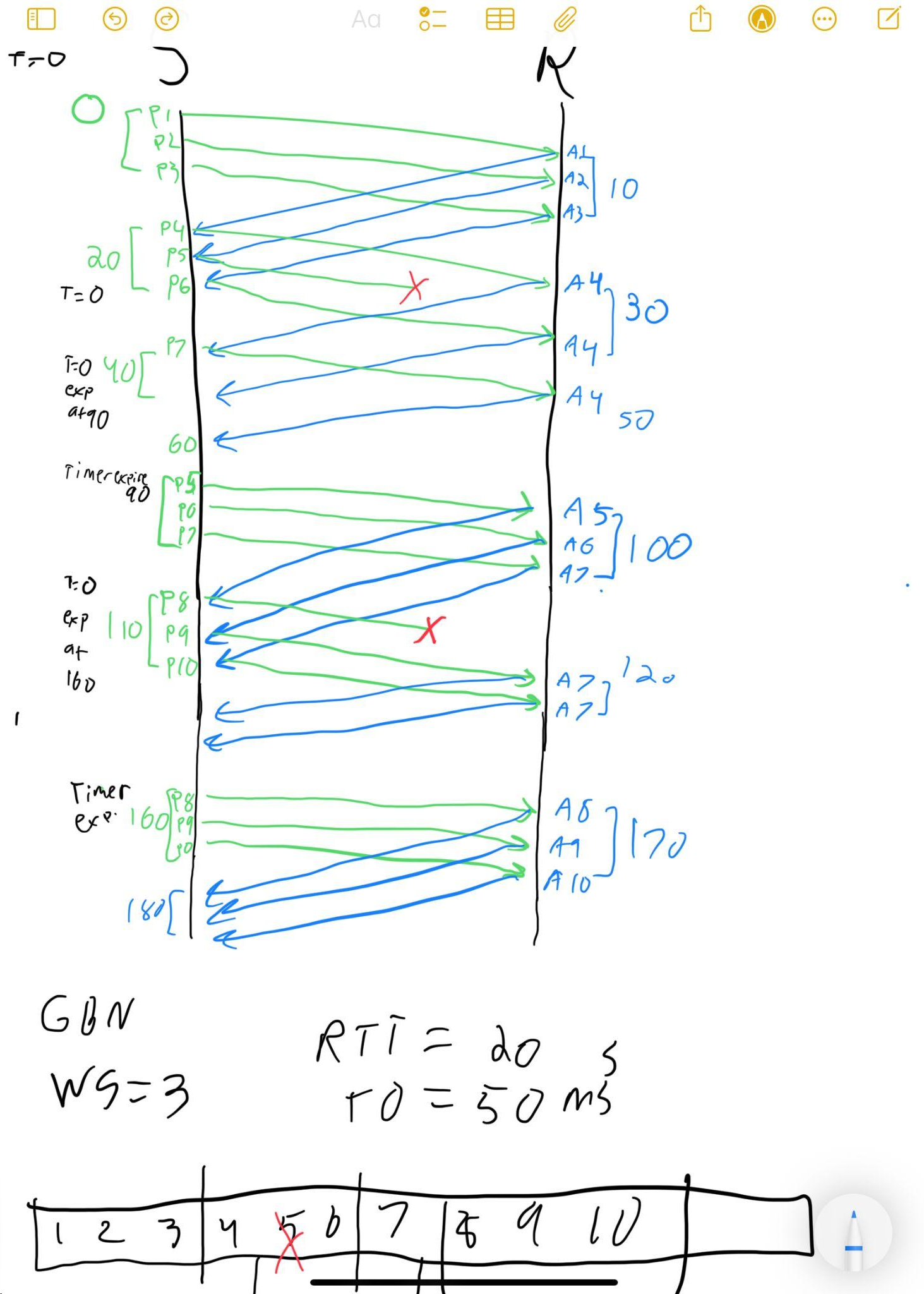
Elaboration: Go-Back-N uses cumulative ACKs and timeouts to detect loss. When packet 5 is lost, the receiver continues to send duplicate ACKs (ACK 4) because subsequent packets are out of order and discarded. The sender’s timeout fires, triggering retransmission from packet 5 onward. The retransmission includes packets 5, 6, 7, and 8; when 8 is lost again, another timeout occurs. This all-or-nothing retransmission can waste bandwidth on high-loss links, motivating the shift to Selective Repeat in modern protocols.
-
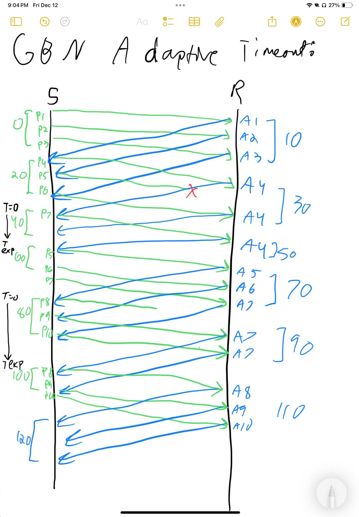
(b) Redo (a) assuming the sender uses the improved Go-Back-N with adaptive timeouts.
Solution
Problem 10: Sender Window Sequence Numbers Analysis
Consider the Go-Back-N protocol with a sender window size of 3. Suppose that at time t, the next in-order packet that the receiver is expecting has a sequence number of k. Assume that the medium does not reorder messages. Answer the following questions:
- (a) What are the possible sets of sequence numbers inside the sender’s window at time t. Justify your answer.
Solution
With window size 3 and receiver NPE = k (expects k next), k has not yet been delivered in order. Thus the sender’s outstanding window lower bound is k. Possible outstanding set is a subset of {k, k+1, k+2}, depending on how many have been sent but not yet ACKed.
Elaboration: This problem explores the constraints imposed by Go-Back-N’s cumulative ACK model. Because the receiver only acknowledges contiguous prefixes of packets, the sender knows that packets up to k-1 have been received in order but packet k may or may not be in flight. The sender’s window must include k and the next two packets to maintain throughput. Similarly, all in-flight ACKs can only acknowledge k-1 or earlier, since the receiver cannot deliver anything beyond k until k arrives.
- (b) What are all possible values of the ACK field in all possible messages currently propagating back to the sender at time t. Justify your answer.
Solution
Only cumulative ACKs for k−1 may be in flight (including duplicates). No ACK ≥ k is possible until k is received in order.
Elaboration: Go-Back-N’s cumulative acknowledgment constraint means the receiver can only ACK the highest contiguous sequence it has received. Since NPE = k, the receiver has not yet delivered packet k, so it cannot acknowledge k or beyond. All in-flight ACKs must be for k−1 or earlier. This creates a tight coupling between receiver state (NPE) and possible network state (in-flight ACKs), which helps the sender infer what the receiver has successfully processed based on ACK arrivals.
Problem 11: Go-Back-N Packet Loss Transmission Count
Host A needs to send a message consisting of 9 packets to host B using a sliding window protocol with a window size of 3. Assume that Go-Back-N is used for reliable packet transfer. All packets are ready and immediately available for transmission. If every 5 th packet that A transmits gets lost but no ACKs from B ever get lost, what is the number of packets that A will transmit to send the message to B? Show your work. (Answer: 16)
Solution
Problem 12: Selective Repeat Packet Loss Transmission Count
Host A needs to send a message consisting of 9 packets to host B using a sliding window protocol with a window size of 3. Assume that Selective Repeat is used for reliable packet transfer. All packets are ready and immediately available for transmission. If every 5 th packet that A transmits gets lost but no ACKs from B ever get lost, what is the number of packets that A will transmit to send the message to B? Show your work. (Answer: 11)
Solution
Problem 13: Go-Back-N Larger Window Packet Loss
Host A needs to send a message consisting of 10 packets to host B using a sliding window protocol with a window size of 4. Assume that Go-Back-N is used for reliable packet transfer. All packets are ready and immediately available for transmission. If every 6 th packet that A transmits gets lost but no ACKs from B ever get lost, what is the number of packets that A will transmit to send the message to B? Show your work. (Answer: 17)
Problem 14: Selective Repeat Larger Window Packet Loss
Host A needs to send a message consisting of 10 packets to host B using a sliding window protocol with a window size of 4. Assume that Selective Repeat is used for reliable packet transfer. All packets are ready and immediately available for transmission. If every 6 th packet that A transmits gets lost but no ACKs from B ever get lost, what is the number of packets that A will transmit to send the message to B? Show your work. (Answer: 11)
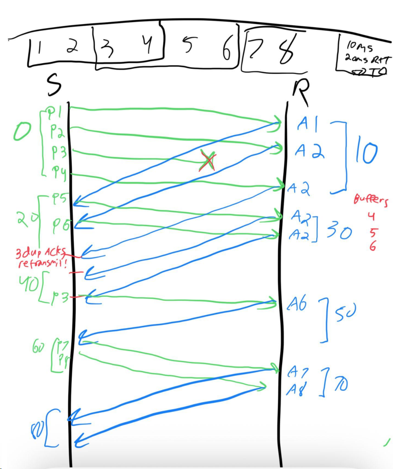
Problem 15: Sliding Window with TCP Fast Retransmit
Consider a sender and receiver employing sliding window protocol with a window size of 4. Assume that the receiver sends cumulative acknowledgements, and the sender employs TCP’s fast retransmit algorithm to recover lost packets. You want to send 8 packets labeled 1 to 8 to the receiver. Take a 10ms one-way delay between the sender and the receiver and a 50ms timeout period.
Elaboration: Fast retransmit is a key optimization in TCP. Instead of waiting for a timeout when a packet is lost, the sender retransmits upon receiving three duplicate ACKs (i.e., four total ACKs with the same sequence number). This allows recovery in roughly one RTT rather than waiting for the timeout. The diagram will show packet 3 being lost, followed by the receiver sending duplicate ACKs for packet 2, and the sender triggering fast retransmit before the timeout fires.
- (a) Assuming that the 3rd packet is lost the first time it is sent, draw a diagram showing when each packet is sent, and the corresponding ACK sent by the receiver in response to each packet.
- (b) Assuming the transmission starts at time 0, at what time does the receiver receive the last packet? Ignore the transmission time for a packet (assume it is 0).
Solution
Problem 16: Reliable Broadcast Channel Protocol
Consider a scenario in which host A wants to simultaneously send messages to hosts B and C. A is connected to B and C via a broadcast channel, i.e., a packet sent by A is carried by the channel to both B and C. Suppose that the broadcast channel connecting A, B and C can independently lose or corrupt packets (and so for example, a packet sent from A might be correctly received by B, but not by C). Design a stop-and-wait-like protocol for reliably transferring a packet from A to B and C, such that A will not send the next packet until it knows that both B and C have correctly received the current packet.
Solution
Answer: A broadcasts each packet and waits until it receives ACKs from both B and C (retransmitting as needed); it advances to the next sequence number only after both ACKs have been received.
Elaboration:
The Core Idea
Since the channel is broadcast, A sends a single packet that “should” go to both B and C. However, because losses are independent, A cannot assume that if B got it, C got it too.
The Rule
Host A acts as if it has two logical “Stop-and-Wait” threads running in parallel but synchronized to the same transmission. It cannot proceed to Packet $N+1$ until both logical threads have confirmed Packet $N$ (i.e., both B and C have ACKed).
1. Sender (Host A) Protocol
Variables:
SeqNum: Current sequence number (0 or 1, alternating).Received_ACK_B: Boolean flag (initially False).Received_ACK_C: Boolean flag (initially False).
Behavior:
-
Send State:
- A creates a packet with sequence number
SeqNum. - A broadcasts the packet to the channel.
- A starts a Timer.
- A creates a packet with sequence number
-
Wait State (Listening for ACKs):
- Event: Received ACK from B
- Mark
Received_ACK_B = True.
- Mark
- Event: Received ACK from C
- Mark
Received_ACK_C = True.
- Mark
- Event: Timer Expires
- If
Received_ACK_BandReceived_ACK_Care NOT BOTH True:- Retransmit the packet.
- Restart the Timer.
- (Note: Even if B already ACKed, A must re-broadcast to reach C. B will just handle the duplicate.)
- If
- Event: Received ACK from B
-
Transition State:
- If (
Received_ACK_B== True) AND (Received_ACK_C== True):- Stop Timer.
- Toggle
SeqNum(0 $\rightarrow$ 1). - Reset flags (
Received_ACK_B = False,Received_ACK_C = False). - Fetch next data and go to Send State.
- If (
2. Receiver (Hosts B and C) Protocol
The receivers behave exactly like a standard Stop-and-Wait receiver. They don’t need to know about each other.
Behavior for Host B (and similarly for C):
-
Wait for Packet:
- Wait for packet from A.
-
Packet Arrives:
- Check for corruption (checksum).
- If Corrupt: Discard. Do nothing.
- If Correct:
- Check Sequence Number.
- If
SeqNum == Expected SeqNum:- Pass data to application.
- Send
ACK(SeqNum)to A. - Increment Expected
SeqNum.
- If
SeqNum == Old/Duplicate SeqNum:- (This happens if A retransmitted because C missed the packet.)
- Discard data (don’t pass to app).
- Send
ACK(SeqNum)to A. (Crucial: A needs to hear this again to know B is still happy.)
Problem 17: Stop-and-Wait vs Sliding Window Protocols
What’s the problem with Stop-and-Wait protocol? Briefly describe how the sliding windows protocols solve the problem.
Solution
Stop‑and‑Wait allows only one outstanding packet, wasting bandwidth on high BDP paths. Sliding windows permit multiple outstanding packets, improving utilization and throughput.
Elaboration: Stop-and-Wait’s fundamental limitation is that the sender must wait for an ACK before sending the next packet. On a high-latency or high-bandwidth link, the sender sits idle for an entire RTT while waiting for the ACK to return. For example, a 1 Gbps link with 100 ms RTT can transmit 100 Mb of data during one RTT, but Stop-and-Wait sends only one packet per RTT, severely underutilizing the link. Sliding windows decouple the RTT from throughput by allowing the sender to transmit multiple packets before waiting for ACKs. The optimal window size equals the bandwidth-delay product: the number of packets that fit in flight during one RTT. This allows full utilization of the link capacity.
Problem 18: TCP Sequence Number Exhaustion
Consider transferring an enormous file of L bytes from host A to host B. Assume an MSS of 1460 bytes.
- (a) What’s the maximum value of L such that TCP sequence numbers are not exhausted? Assume that the TCP sequence numbers start from 0 and recall that TCP sequence number field has four bytes.
Solution
With a 32‑bit sequence space, maximum distinct bytes before wrap‑around is $2^{32}$ bytes (≈ 4.29×10^9).
Elaboration: TCP’s 32-bit sequence number field can represent 2^32 distinct byte positions (0 through 4,294,967,295). Each byte in the stream gets a unique sequence number, so the maximum file size without sequence number wrap-around is exactly 2^32 bytes or about 4.29 GB. Beyond this size, sequence numbers wrap back to 0, which can cause ambiguity unless proper sequence number arithmetic and timing constraints are maintained. Modern high-speed networks often require TCP extensions to handle wrap-around safely.
- (b) Consider sending a 1MB file. How long does it take to transmit this file. Assume that a total of 66 bytes of transport, network, and data-link headers are added to each segment before the resulting packet is sent out over a 10Mbps link. Ignore flow and congestion control so A can pump out the segments back-to-back and contiguously.
Solution
Segment payloads of 1460 bytes → 1,000,000 / 1460 ≈ 684 full segments + 1 remainder (1360 bytes). Per‑packet overhead = 66 bytes.
- Total bytes on the wire ≈ 684×(1460+66) + (1360+66) = 1,045,210 bytes.
- Bits ≈ 1,045,210 × 8 = 8,361,680 bits.
- Time at 10 Mbps ≈ 8,361,680 / 10,000,000 ≈ 0.836 s.
Elaboration: This calculation shows the overhead of protocol headers in network transmission. The 1MB application data requires 66 bytes of headers per packet (TCP, IP, and link-layer headers), adding about 4.5% overhead. The segmentation into 684 full packets plus one partial packet reflects TCP’s MSS constraint. On a 10 Mbps link, the limiting factor is transmission time, not processing or propagation delays. This analysis helps network engineers estimate bandwidth requirements and understand the relationship between application data size and actual network utilization.
Problem 19: Go-Back-N vs Selective Repeat Comparison
Go-Back-N and Selective-Repeat are retransmission strategies with sliding window protocols. Describe and discuss the advantages of each. How does using one or the other change the requirements for buffers in the sending and receiving windows?
Solution
- GBN: simpler receiver; retransmits from first loss onward; wastes bandwidth on single losses; receiver buffer minimal; sender buffers up to window.
- SR: retransmits only lost packets; higher throughput on lossy links; requires out‑of‑order buffering at receiver (≈ window size); per‑packet timers add complexity.
Elaboration: GBN’s simplicity comes from requiring only cumulative ACKs and a single sender-side timer. The receiver can discard out-of-order packets (saving buffer space) and simply duplicate-ACK the highest in-order sequence. However, on lossy links, a single loss triggers retransmission of the entire window, wasting bandwidth. SR avoids this by allowing selective retransmission: the receiver ACKs individual packets and buffers out-of-order arrivals, and the sender retransmits only the missing packet. This efficiency comes at a cost: the receiver needs a buffer of size ≈ window for out-of-order storage, each packet needs its own timer at the sender, and implementation is more complex. Modern protocols like TCP (which uses a form of SR with SACK) and QUIC prefer SR for high-speed, lossy links.
Problem 20: Optimal Sliding Window Size Calculation
Host A uses 32 byte packets to transmit a message to host B using the sliding window protocol. The RTT between A and B is 80 milliseconds and the bottleneck bandwidth on the path between A and B is 128Kbps. What is the optimal window size that A should use? Show your work. (Answer: 40).
Solution
Optimal window ≈ bandwidth–delay product in packets:
- BDP = RTT × bandwidth = 0.08 s × 128,000 bps = 10,240 bits.
- Packet size = 32 bytes = 256 bits.
- Window = 10,240 / 256 = 40 packets.
Elaboration: The bandwidth-delay product (BDP) represents the total number of bits that can be “in flight” across the network at any given time. With a 128 Kbps link and 80 ms RTT, the network can hold 10,240 bits. The sender should always have this amount of data in flight to keep the pipe full and achieve maximum throughput. A window smaller than BDP/packet-size will leave the link idle (underutilization); a window larger than BDP won’t improve throughput (and will unnecessarily buffer packets in the network). This calculation is critical for link capacity planning and helps explain why high-speed, long-distance networks (e.g., intercontinental transfers) require large TCP windows—the BDP is enormous.
Problem 21: Optimal Window Size Formula
The distance between two hosts A and B is L kilometers. All packets are K bits long. The propagation time per kilometer is t seconds. Let R bits/sec be the channel capacity. Assume that A and B use the sliding window protocol for reliable packet deliver. Assuming that the processing and queuing delay is negligible, what’s the optimal window size that A should use? Show your work. (Answer: (2LtR)/K)
Solution
Optimal window equals the bandwidth–delay product in packets:
- One‑way propagation time = $L\,t$; RTT ≈ $2Lt$.
- Bits in flight = $\text{RTT} \times R = 2LtR$.
- Packets = $\dfrac{2LtR}{K}$.
Problem 22: Flow Control via Delayed ACKs
Consider combining TCP’s reliable packet delivery, i.e., sliding window protocol, with its flow control mechanism as follows: The receiver delays ACKs, that is, not send the ACK until there is a free buffer space to hold the next frame. In doing so, each ACK would simultaneously acknowledge the receipt of the last frame and tell the source there is now a free buffer space available to hold the next frame. Explain why implementing flow control in this way is NOT a good idea.
Solution
Delaying ACKs hides successful delivery from the sender. Without timely ACKs, the sender’s timeout fires and triggers needless retransmissions, wasting bandwidth and increasing latency. Flow control should be signaled via advertised window, not by withholding ACKs.
Elaboration: This approach confuses TCP’s reliability and flow control mechanisms. ACKs serve dual purposes: confirming packet delivery and advertising buffer space. Delaying ACKs until buffer space opens conflates these functions, causing the sender to interpret delayed ACKs as packet loss rather than flow control. The result is spurious retransmissions and reduced performance. TCP’s proper approach separates concerns: ACKs confirm delivery promptly, while the advertised window field explicitly signals buffer availability. This allows the receiver to throttle the sender (window = 0) while still acknowledging received data.
Problem 23: TCP Zero Window Probing
A sender on a TCP connection that receives a 0 advertised window periodically probes the receiver to discover when the window becomes nonzero. Why would the receiver need an extra timer if it were responsible for reporting that its advertised window had become nonzero (i.e., if the sender did not probe)?
Solution
To avoid deadlock. If the sender isn’t probing and an ACK indicating a nonzero window is lost, the receiver must use a timer to retransmit the window‑update notification; otherwise both sides could wait indefinitely.
Elaboration: This deadlock scenario occurs when the receiver’s window opens (buffer space becomes available) and it sends a window update, but that update is lost in transit. Without sender-driven probing, the sender waits forever for a window update that will never be retransmitted, while the receiver waits forever for data that will never be sent. The receiver needs a timer to periodically resend window updates until acknowledged, or the sender needs to probe with zero-window probes. TCP chooses sender-driven probing because it’s simpler: only one entity (sender) needs the timer, and the probe frequency can adapt to network conditions.
Problem 24: TCP Memory Allocation Effects
Assume that an operating system can give more memory to, or request memory back from, a TCP connection, based on memory availability and the connection’s requirements. (a) What would be the effects of the memory available to a connection? (b) What about reducing the memory for the connection?
Solution
(a) More memory enlarges send/receive buffers, allowing a larger advertised window and higher throughput on high‑BDP paths. (b) Less memory shrinks buffers, reducing the advertised window and throughput; the sender must pace to avoid overrunning the smaller window.
Elaboration: Reduced memory forces smaller buffers, which constrains the advertised window and limits throughput. On high-BDP paths, small windows severely underutilize link capacity. The sender’s transmission rate becomes limited by the receiver’s buffer size rather than network capacity. This creates a feedback loop: smaller windows lead to lower throughput, which may actually be appropriate during memory pressure to avoid overwhelming the receiver’s processing capabilities. Modern operating systems dynamically adjust TCP buffer sizes based on available memory and connection requirements.
Problem 25: Sliding Window Packet Arrival Sequence
Consider a sliding-window reliable delivery protocol that uses timeouts and cumulative ACKs as in TCP. Assume that the sender’s and receiver’s window size is 4, i.e., at most 4 packets can be buffered by the receiver and at most 4 unACKed packets can be sent by the sender. Further assume that the receiver has received all packets up to packet number 7 and is expecting packet number 8, i.e., Next Packet Expected
(NPE) = 8 and the Last Packet Acceptable (LPA) is 11. Suppose the receiver receives the following packets 8, 11 9 10 12 13 in this order. Show the values of Next Packet Expected (NPE) and Last Packet Acknowledged (LPA) after each packet arrival. Also describe whether an ACK is sent to sender after each packet arrival and if so write down the sequence number of the packet that is ACKed.
| Event | Action | NPE | LPA |
|---|---|---|---|
| Initial Condition | 8 | 11 | |
| Packet 8 arrives | Send ACK for 8 | 9 | 12 |
| Packet 11 arrives | Buffer 11, Send ACK for 8 | 9 | 12 |
| Packet 9 arrives | Send ACK for 9 | 10 | 13 |
| Packet 10 arrives | Send ACK for 11 | 12 | 15 |
| Packet 12 arrives | Send ACK for 12 | 13 | 16 |
| Packet 13 arrives | Send ACK for 13 | 14 | 17 |
Solution
The table shows cumulative ACK behavior with receiver window size 4: out‑of‑order arrivals are buffered; ACKs reflect the highest contiguous sequence received (8→11), then jump when missing packets arrive (ACK 11 after 10), advancing NPE and LPA accordingly.
Elaboration: This problem demonstrates TCP’s sliding window operation with buffering and cumulative acknowledgments. The receiver maintains a window [NPE, LPA] and can buffer out-of-order packets within this range. When packet 8 arrives, it’s the expected sequence, so NPE advances to 9 and an ACK is sent. Packet 11 arrives out of order and is buffered, but NPE remains 9 (still waiting for 9 and 10). When packets 9 and 10 finally arrive, they enable delivery of the buffered sequence 8-11, causing NPE to jump to 12 and LPA to advance accordingly. This buffering improves performance by avoiding unnecessary retransmissions of correctly received but out-of-order packets.
Problem 26: TCP Zero Window Probing Timer
A sender on a TCP connection that receives a 0 advertised window periodically probes the receiver to discover when the window becomes nonzero. Why would the receiver need an extra timer if it were responsible for reporting that its advertised window has become nonzero (i.e., if the sender did not probe)?
Solution
Same rationale as Problem 23: the receiver needs a timer to retransmit its window‑opening notification if the prior update was lost, ensuring progress without sender probes.
Elaboration: This problem highlights a critical design choice in TCP’s zero-window handling. If the receiver were responsible for advertising window openings (rather than the sender probing), the receiver would need to implement a retry mechanism for window update messages. Without this, a lost window-opening ACK creates deadlock: the receiver thinks it has notified the sender that space is available, but the sender never received this notification. Implementing receiver-driven window updates would require additional timer management, state tracking, and retransmission logic at the receiver—adding complexity compared to TCP’s simpler sender-driven probe approach.
Problem 27: TCP Sequence Number Wrap Around
The TCP sequence number field in the TCP header is 32 bits long, which is big enough to cover 4 billion bytes data. Even if this many bytes were never transferred over a single connection, why might the sequence number still wrap around from 232 - 1 to 0.
Solution
Sequence numbers are modulo $2^{32}$. On long‑lived connections or high rates, the sender can cycle through the 32‑bit space even if the application’s total data is below $2^{32}$, leading to natural wrap‑around.
Elaboration: While $2^{32}$ bytes (4 GB) seems enormous, modern high-speed links can exhaust this space within seconds. For example, a 10 Gbps link sending maximum-sized segments will wrap around in about 3.4 seconds. TCP handles wrap-around through sequence number arithmetic (modulo $2^{32}$), which works correctly as long as sequence numbers don’t wrap around within the maximum segment lifetime (MSL). The MSL (typically 2 minutes) bounds how old segments can be; TCP’s timestamp option (RFC 1323) further protects against wrap-around issues and is essential for modern high-speed links.
Problem 28: Sliding Window Protocol Field Sizing
You are hired to design a reliable byte-stream protocol that uses a sliding window (like TCP). This protocol will run over a 100-Mbps network. The RTT of the network is 100ms, and the maximum segment lifetime is 60 seconds. How many bits would you include in the AdvertisedWindow and SequenceNum fields of your protocol.
Solution
- AdvertisedWindow: BDP = 0.1 s × 100,000,000 bps = 10,000,000 bits = 1,250,000 bytes → need ≥ 1.25 MB; $2^{20} \approx 1$ MB, $2^{21} \approx 2$ MB → 21 bits.
- SequenceNum: bytes that might be outstanding within MSL = $(100\,\text{Mbps} \times 60\,\text{s})/8 \approx 750{,}000{,}000$ bytes; $2^{29} \approx 536$M, $2^{30} \approx 1{,}073$M → 30 bits.
Elaboration: The AdvertisedWindow field must cover the BDP—the maximum bytes in flight. The SequenceNum field must avoid wrap-around within MSL: if a late-arriving segment from a previous connection instance carries a recycled sequence number, the receiver must not confuse it with a current segment. Standard TCP uses 32 bits for both fields; this problem demonstrates why high-bandwidth or high-latency links (intercontinental, satellite) need extensions like RFC 1323 timestamp options to safely handle sequence number space and large windows.
Problem 29: TCP Congestion Window with Fast Retransmit
Sketch the TCP congestion window size as a function of time (measured in RTTs) if a single loss occurs on the 12th packet. Assume that the system uses fast retransmission.
Solution
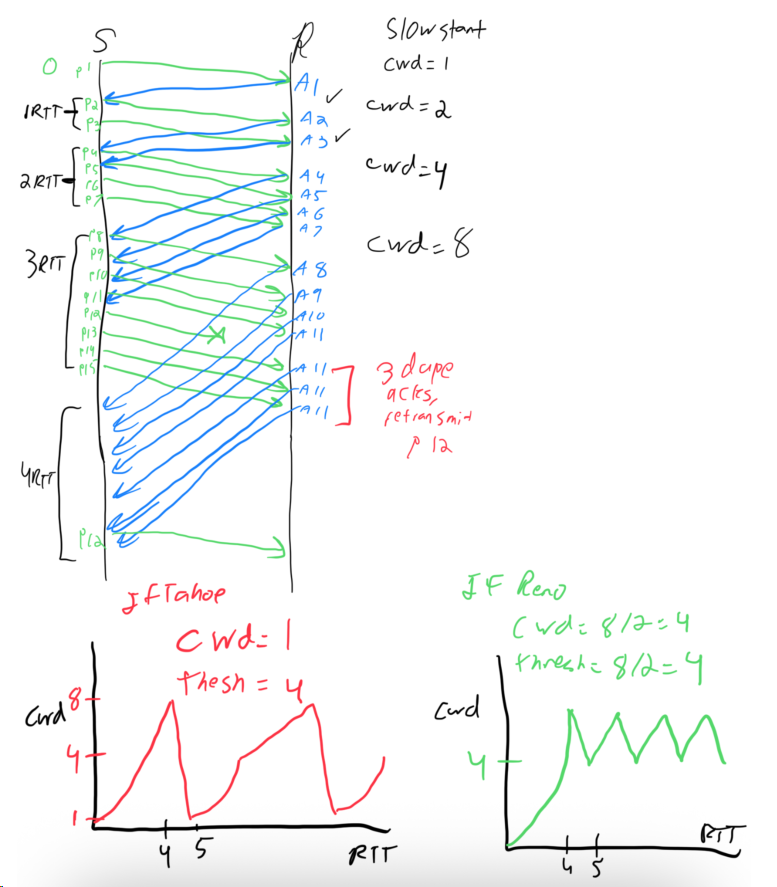
Elaboration: The graph shows the characteristic TCP Reno sawtooth pattern: slow-start (exponential growth) until loss, then fast retransmit halves the window and enters congestion avoidance (linear growth), avoiding the drastic reset-to-1 that a timeout would cause. Fast retransmit relies on receiving 3 duplicate ACKs, which signals isolated loss rather than network collapse; this allows faster recovery and better throughput than timeout-based recovery on lossy links.
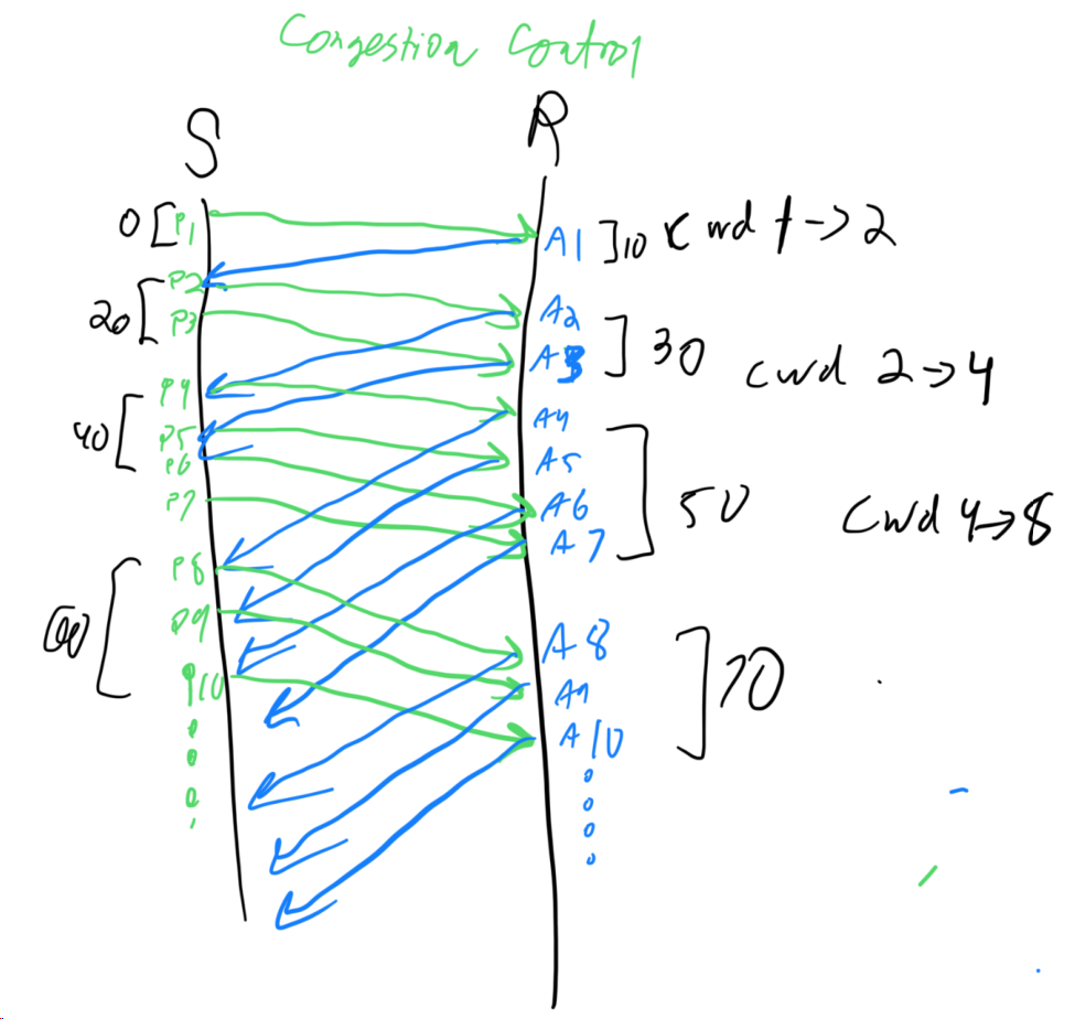
Problem 30: Flow Control and Congestion Control Timing
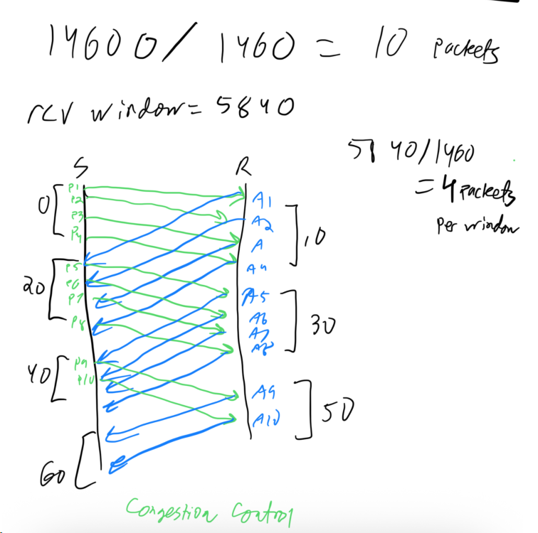
Assume that you want to send 14600 bytes of data to a TCP receiver. Further assume that during connection establishment, the TCP receiver exports a receive window of size 5840. Also assume that MSS is 1500 bytes, IP header is 20 bytes and TCP header is 20 bytes. Thus you can put 1460 bytes of application data to each TCP packet.
- (a) Assume that TCP congestion control is not employed, but the flow control is employed. Assuming no packet drops, sketch when each packet is sent by the sender. Assume a one-way delay of 10 ms and that the transmission starts at time 0. At what time does the receiver application receive the last byte of the data?
- (b) Assume now that TCP congestion control is also employed, and the congestion window starts from 1 packet. Assuming no packet drops, sketch when each packet is sent by the sender. Assume a one-way delay of 10 ms and that the transmission starts at time 0. At what time does the receiver application receive the last byte of the data?
Solution
Problem 31: Congestion Control Threshold Update
Consider a TCP connection with a current congestion window size of 10.
- (a) Assume that a packet loss is detected by 3 duplicate ACKs. What would be the new value of ssthresh and congestion window? Would the congestion window increase linearly or exponentially in the next time slot?
Solution
Fast retransmit/fast recovery: set
ssthresh = cwnd/2 = 5; setcwnd = ssthresh = 5. Subsequent growth is linear (congestion avoidance).Elaboration: TCP Reno’s fast recovery avoids aggressive window reduction. By halving cwnd instead of resetting to 1 (as timeout does), TCP maintains reasonable throughput and avoids the slow-start ramp-up penalty. The 3 duplicate ACKs indicate isolated packet loss, not congestion collapse, so moderate reduction is appropriate. Linear growth in congestion avoidance probes the link capacity carefully before the next loss, making TCP Reno much more efficient than earlier versions on lossy but not-congested links.
- (b) Assume that a packet loss is detected by a timeout. What would be the new value of ssthresh and congestion window? Would the congestion window increase linearly or exponentially in the next time slot?
Solution
Timeout: set
ssthresh = cwnd/2 = 5; setcwnd = 1 MSS(slow start). Subsequent growth is exponential untilcwndreachesssthresh.Elaboration: Timeout is TCP’s conservative response, signaling possible severe congestion or network outage. Resetting cwnd to 1 and re-entering slow-start causes throughput to drop dramatically but ensures the sender backs off aggressively. The exponential ramp-up allows probing for available capacity without overwhelming a congested network. This conservative behavior is why timeouts are feared: they can reduce a 10 Mbps flow to kilobits/second, taking multiple RTTs to recover. Modern congestion control algorithms (like CUBIC or BBR) aim to recover faster from timeouts while remaining fair.
Problem 32: Extended TCP Window Scaling Performance
Recall the proposed TCP extension that allows flow control window sizes much larger than 64KB. Suppose that you are using this extended TCP over a 1-Gbps link with a latency of 100ms to transfer a 10-MB file, and the TCP receive window size is 1MB. If TCP sends 1-KB packets, assuming no congestion and no lost packets.
- (a) How many RTTs does it take until the send window reaches 1MB? (Recall that the window is initialized to the size of a single packet.)
Solution
Slow start doubles each RTT: $2^{10} = 1024$ KB → 10 RTTs.
Elaboration: This exponential growth is the hallmark of slow-start: cwnd = 1, 2, 4, 8, 16, … packets each RTT. While “slow” in name, it’s aggressive in practice—exponential growth reaches 1MB in just 10 RTTs (or 1 second here). This is the key disadvantage for high-BDP links: even with large receive windows, slow-start must ramp up for many RTTs before utilizing the link. On a 100-millisecond RTT link needing 1 MB window, the sender wastes 1 second ramping up, delivering poor throughput for short flows. This motivated initial congestion window (IW) increases (from 3 to 10 packets) and modern algorithms like CUBIC that accelerate ramp-up.
- (b) How many RTTs does it take to send the file?
Solution
First 10 RTTs send $1+2+4+\dots+512=1023$ KB. Remaining $10{,}000 - 1{,}023 = 8{,}977$ KB at 1 MB/RTT → 9 RTTs. Total = 10 + 9 = 19 RTTs.
- (c) If the time to send the file is given by the number of required RTTs multiplied by the link latency, what’s the effective throughput for the transfer? What percentage of the link bandwidth if utilized?
Solution
Link latency = 100 ms. Time = $19 \times 0.1 = 1.9$ s. Throughput ≈ $10\,\text{MB}/1.9 \approx 5.26$ MB/s. Link capacity = 1 Gbps ≈ 125 MB/s → utilization ≈ $5.26/125 \approx 4.21\%$.
Elaboration: Only 4.2% of the link capacity is utilized despite no packet loss or congestion! The bottleneck is slow-start’s startup phase: 10 RTTs (1 second) deliver only 1 MB, then 9 RTTs deliver the remaining 9 MB at full window speed. For short transfers (< 100 RTTs), slow-start overhead dominates, severely underutilizing high-BDP links. This motivates techniques like TCP Fast Open, larger initial congestion windows, and application-level solutions (HTTP/2 multiplexing, persistent connections). On satellite links with 500+ ms RTTs, even sending a single file suffers similar inefficiency.
Problem 33: UDP vs TCP Single Byte Transfer Latency
Consider two hosts A and B separated by a one-way delay of 10ms. Assume that B runs a server and A runs a client. Assume that the client application running at host A wants to send 1 byte to the server.
- (a) Assume that the client and the server communicate over UDP, and no UDP packet is lost in the network. What is the minimum amount of time it would take for the server to receive the packet, after the client starts running? Justify your answer.
Solution
One data trip: 10 ms (no handshake).
Elaboration: UDP’s connectionless model eliminates handshake overhead. The client simply sends a datagram directly; there’s no 3-way handshake, no state setup, no acknowledgment required. This 10 ms one-way delay is the absolute minimum for any transport on this link. However, the server has no assurance the packet arrived, no reliability guarantees, and no flow control. UDP’s ultra-low latency makes it ideal for time-sensitive applications (gaming, voice, VoIP, real-time streaming) where timeliness matters more than perfection. TCP’s 3-way handshake cost (30 ms) is the price of reliability.
- (b) Assume that the client and the server communicate over TCP, and no TCP packet is lost in the network. What is the minimum amount of time it would take for the server to receive the packet, after the client starts running? Justify your answer.
Solution
TCP handshake + data: SYN at 0 ms → SYN‑ACK at 10 ms → ACK+data at 20 ms → server receives data at 30 ms.
Elaboration: TCP’s 3-way handshake adds 2 RTTs of latency before data flows. The client must wait for the server’s SYN-ACK before sending data (since TCP guarantees order and reliability). This 30 ms overhead is significant for low-latency applications. Newer protocols like QUIC and protocols with TCP Fast Open (TFO) attempt to reduce this by allowing data piggybacking on the handshake, achieving 1 RTT latency. For massive file transfers, the handshake cost (30 ms) is negligible, but for millions of short transactions or latency-critical games, TCP’s overhead becomes prohibitive. This motivates HTTP/3 (QUIC), which combines UDP’s speed with TCP’s reliability through cryptographic handshakes and connection IDs.
Problem 34: TCP Reno Congestion Window Analysis
Consider the following plot of TCP window size as a function of time:
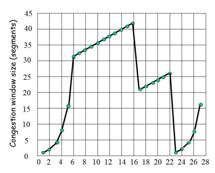
Assuming TCP Reno is the protocol experiencing the behavior shown in the graph, answer the following questions. In all cases a short discussion justifying the answer is provided.
-
(a) Identify the intervals of time when TCP slow start is operating.
-
(b) Identify the intervals of time when TCP congestion avoidance is operating.
-
(c) After the 16th transmission round, is segment loss detected by a triple duplicate ACK or by a timeout?
-
(d) After the 22nd transmission round, is segment loss detected by a triple duplicate ACK or by a timeout?
-
(e) What’s the initial value of Threshold at the first transmission round?
-
(f) What’s the value of Threshold at the 18th transmission round?
-
(g) What’s the value of Threshold at the 24th transmission round?
-
(h) During what transmission round is the 70th segment sent?
-
(i) Assuming a packet loss is detected after the 27th round by three receipts of a triple duplicate ACK, what will be the values of the congestion-window size and of Threshold?
Problem 35: RTT Variance Impact on Congestion Control
In TCP (Jacobson) congestion control, the variance in round-trip times for packets implicitly influences the congestion window. Explain how a high variation in the round-trip time affects the congestion window. What is the impact of this high variation on the throughput for a single connection?
Solution.
Higher RTT variation increases the deviation term DevRTT, which raises the retransmission timeout TimeoutInterval = EstimatedRTT + 4·DevRTT. More conservative timeouts reduce spurious retransmissions but slow recovery. Jitter can also cause spurious timeouts (if the estimate lags), triggering multiplicative decreases of cwnd. Net effect: slower cwnd growth, more conservative behavior, and lower throughput for a given path.
Elaboration: TCP’s timeout calculation is deliberately conservative: TimeoutInterval = EstimatedRTT + 4*DevRTT adds four standard deviations of margin. High jitter (variance) inflates DevRTT, which raises the timeout threshold, meaning TCP waits longer before declaring loss. This conservatism prevents spurious retransmissions from good packets that are merely delayed. However, on highly variable paths (e.g., cellular, wifi), packets legitimately delayed 2-3x their average RTT may never trigger timeout, paradoxically causing TCP to underestimate loss and grow cwnd recklessly—then sudden loss triggers recovery. Modern algorithms (like CUBIC and BBR) use packet loss as the primary congestion signal rather than timeout, making them less sensitive to RTT jitter.
Problem 36: Flow Control vs Congestion Control Bottleneck
Host A is sending an enormous file to host B over a TCP connection. Over this connection, there is never any packet loss, and the timers never expire. Denote the transmission rate of this link connecting host A to the Internet by $R$ bps. Suppose that the process in host A is capable of sending data into its TCP socket at a rate of $S$ bps, where $S = 10R$. Further suppose that the TCP receive buffer is large enough to hold the entire file, and the send buffer can only hold one percent of the file. What would prevent the process in host A from continuously passing data to its TCP socket at $S$ bps. TCP flow control? TCP congestion control? Or something else?
Solution
The bottleneck is the path capacity $R$ (and the socket/send buffer pacing). Flow control isn’t limiting (receiver buffer is large), and congestion control won’t reduce rate without loss; the NIC/link rate caps throughput near $R$, so the application cannot sustain $S=10R$.
Elaboration: This problem highlights an often-overlooked constraint: the physical link capacity. Flow control (receiver advertised window) is irrelevant because the receiver buffer is huge. Congestion control is irrelevant because there’s no loss, so cwnd grows unchecked to a very large value. What actually limits the sender is the network interface card (NIC) and the physical link: they cannot transmit faster than $R$ bps, period. The send buffer (holding 1% of the file) fills up quickly because the application produces data at $10R$ but the NIC drains it at only $R$. The OS blocks the application’s send calls when the send buffer fills, naturally throttling the application to the link rate. This is an important distinction: TCP’s mechanisms (flow control, congestion control) cooperate with the physical layer’s hard limit, not replace it.
Problem 37: TCP RTT Estimation Exponential Moving Average
Consider the TCP procedure for estimating RTT. Suppose that $\alpha = 0.1$. Let $SampleRTT_1$ be the most recent sample RTT, let $SampleRTT_2$ be the next most recent sample RTT and so on.
-
(a) Given a TCP connection, suppose 4 ACKs have been received with corresponding sample RTTs $SampleRTT_4, SampleRTT_3, SampleRTT_2,$ and $SampleRTT_1$. Express $EstimatedRTT$ in terms of the four sample RTTs.
-
(b) Generalize your formula for $n$ sample round-trip times.
-
(c) For the formula in part (b), let $n$ approach infinity. Comment on why this averaging procedure is called an exponential moving average.
Solution.
- (a) With $\alpha = 0.1$ and letting $SampleRTT_1$ be most recent: $EstimatedRTT \approx 0.1\,SampleRTT_1 + 0.9\cdot0.1\,SampleRTT_2 + 0.9^2\cdot0.1\,SampleRTT_3 + 0.9^3\cdot0.1\,SampleRTT_4$ (ignoring any initial baseline term).
- (b) In general (most recent index 1): $EstimatedRTT_n = (1-\alpha)^n\,EstimatedRTT_0 + \sum_{i=1}^{n} \alpha\,(1-\alpha)^{i-1}\,SampleRTT_i$. For large $n$ or negligible $EstimatedRTT_0$, the sum dominates.
- (c) Weights decay geometrically by factor $(1-\alpha)$ with sample age; older samples’ influence shrinks exponentially and the weights sum to 1 in the limit — hence “exponential moving average.”
Elaboration: The choice of $\alpha = 0.1$ means recent samples get 10% weight and historical estimates get 90% weight. This is relatively conservative, favoring stability over fast reaction. Higher $\alpha$ (e.g., 0.5) reacts faster to RTT spikes but risks instability; lower $\alpha$ (e.g., 0.05) smooths out jitter but lags in truly changing RTT. The exponential form is elegant: old samples automatically decay without explicit pruning, and the formula remains O(1) in memory and computation. TCP implementations use the same principle for DevRTT (variance), tuning both to balance responsiveness and robustness.
Problem 38: TCP File Transfer with Flow and Congestion Control
Consider a TCP client that wants to establish a connection to a TCP server and send a file of size 8192 bytes. Assume that the RTT between the client and the server is 20ms, the MSS is 1024 bytes and the server’s receive buffer size is 3072. Further assume that the initial sequence number selected by the client during connection establishment is 4099, and that no packets are lost during transmission.
-
(a) Assume that TCP employs flow control but not congestion control, draw the packet flow diagram between the client and the sender. Further assume that delayed ACK is not used, i.e., a received packet is ACKed immediately. Label each packet and ACK with a sequence number. Assuming that the client starts at time 0, compute when the server receives the last byte of the packet.
-
(b) Now assume that TCP employs both flow control and congestion control. Draw the packet flow diagram between the client and the sender. Further assume that delayed ACK is not used, i.e., a received packet is ACKed immediately. Label each packet and ACK with a sequence number. Also show the size of the congestion window when an ACK is received. Assuming that the client starts at time 0, compute when the server receives the last byte of the packet.
Problem 39: TCP Segment Loss and Acknowledgement Numbers
Suppose host A sends four TCP segments back-to-back to host B over a TCP connection. The first segment has sequence number 90; the second has sequence number 110, the third has sequence number 170 and the fourth has sequence number 250.
- (a) How much data is in the first, second and third segments?
Solution
First: 110−90 = 20 bytes; Second: 170−110 = 60 bytes; Third: 250−170 = 80 bytes.
Elaboration: TCP sequence numbers represent byte positions in the stream, not packet numbers. The data size of each segment equals the difference between consecutive sequence numbers. For example, segment 1 starts at byte 90 and segment 2 starts at byte 110, so segment 1 contains 20 bytes of application data. This byte-oriented numbering allows TCP to flexibly segment data: the same application data could be split differently (e.g., one 160-byte segment instead of 20+60+80) without changing the sequence number semantics.
- (b) Suppose that the first, third and fourth segments make it to B but the second segment is lost. In the acknowledgements to segments first, third and fourth that host B sends to host A, what will be the acknowledgement number?
Solution
Cumulative ACK remains 110 (next expected byte), since the second segment was lost.
Elaboration: TCP uses cumulative ACKs: an ACK number means “all bytes up to this number have been received in order.” When segment 2 is lost, the receiver can acknowledge segment 1 (110) but not segment 3 or beyond, because segment 3’s data is out-of-order and cannot be delivered to the application until the gap is filled. The receiver buffers segments 3-4 out-of-order but repeatedly sends ACK 110, signaling “I’m still waiting for byte 110.” The sender retransmits segment 2 (via timeout or fast retransmit after 3 duplicate ACK 110s). Once segment 2 arrives, the receiver can immediately ACK all buffered data (up to 330), advancing the window dramatically. This inefficiency (repeated duplicate ACKs) motivated the SACK (Selective ACK) option (RFC 2018), which allows the receiver to explicitly list out-of-order gaps, enabling the sender to retransmit only the missing segment.